
HC-05 QoS Benchmarking with an Elegoo Uno R3: Theory, Implementation, and Results
This post documents the design, implementation, debugging, and analysis of a small but meaningful wireless telemetry benchmark built around an HC-05 Bluetooth serial module and an Elegoo Uno R3. The purpose of the experiment was not simply to prove that Bluetooth communication worked, but to characterize the behavior of the full end-to-end link under controlled conditions and to produce data that could later support comparisons across distances, obstacles, baud rates, or even different development boards.
The final system under test was:
Ubuntu 20.04 host → Bluetooth RFCOMM / SPP link → HC-05 → UART → Uno firmware → UART → HC-05 → Bluetooth RFCOMM / SPP link → Ubuntu 20.04 host
That full round-trip path is the actual object of study. The benchmark therefore measures more than just the radio. It captures the combined behavior of the Bluetooth session, the HC-05 serial bridge, the Uno UART path, the embedded packet parser, and the host-side Python timing logic.
The project began as a simpler communication exercise, but the work described here focuses on the current experiment: a structured QoS-style benchmark designed to measure latency, variability, throughput efficiency, and reliability under repeatable conditions.
Motivation
The main motivation for this experiment was to move from “it works” to “how well does it work?” A Bluetooth-controlled LED demo is a useful functional check, but it does not answer engineering questions such as:
- How much delay does the link introduce?
- How much does that delay vary?
- Does payload size matter?
- Does distance matter more than a light obstacle?
- Does the link degrade by dropping packets, by adding latency, or by becoming less predictable?
Those questions matter because telemetry links are often evaluated only at the level of anecdotal usability. In contrast, a benchmark built around structured packets and controlled timing produces evidence that can support later design decisions.
This experiment was therefore framed as a baseline QoS study. The goal was to quantify four metrics under several controlled conditions: round-trip time (RTT), jitter, packet loss, and goodput.
Theory behind the benchmark
The HC-05 exposes the Bluetooth Serial Port Profile (SPP), which is designed to emulate a serial cable over RFCOMM. On the embedded side, the module presents a UART interface. That means the communication system behaves like a wireless serial bridge rather than a packet-oriented IP link. In practical terms, this is why the benchmark uses a structured binary packet format and an echo-based workflow rather than something like ping or an application protocol intended for TCP/IP.
The most useful metric for a first benchmark is round-trip time. Ubuntu sends a packet, the Uno echoes it back unchanged, and Ubuntu measures the elapsed time. This is attractive because it avoids the need to synchronize clocks between the host and the microcontroller.
For packet i,
RTT(i) = t_receive(i) - t_send(i)
where both timestamps are recorded on the Ubuntu side.
The second metric is jitter, which in this experiment is defined as the standard deviation of RTT within a test condition. A link can have a reasonable average RTT and still behave poorly if the response time is highly variable. Jitter therefore captures timing stability rather than just raw delay.
The third metric is packet loss. A packet is counted as failed if the host does not receive a valid echoed response before timeout, or if the returned packet fails validation because the sequence number, length, checksum, or payload content does not match the original packet.
The fourth metric is goodput, which is more useful than raw line rate because it reflects successfully returned application payload bytes rather than protocol overhead. In this benchmark,
goodput = successfully returned payload bytes / total condition runtime
Taken together, these four metrics allow the system to be characterized in a practical and interpretable way.
Experimental design
The experiment used a stop-and-wait echo design. The Ubuntu host sent one packet, waited for the echoed response, validated it, logged the result, and only then sent the next packet. This design was chosen intentionally. It keeps the relationship between send and receive events unambiguous, simplifies timing interpretation, and makes debugging substantially easier than a streaming or pipelined design would.
The independent variable in the first phase of the benchmark was payload size. The four tested payload sizes were 1 byte, 8 bytes, 32 bytes, and 64 bytes. Those values were chosen because they are small enough for the Uno and HC-05 to handle easily while still being large enough to show how fixed per-packet overhead changes with useful payload size.
The environmental conditions tested were:
- 1 m baseline
- 3 m
- 5 m
- Wood wall condition
The wall condition used a simple interior wood wall in a house. It should therefore be interpreted as a light indoor obstacle rather than a severe attenuation case such as brick, concrete, or metal.
Each condition used 100 trials per payload size, giving 400 packet exchanges per condition.
System under test
The hardware used in the benchmark was intentionally simple:
- Elegoo Uno R3
- HC-05 Bluetooth module
- breadboard and jumper wires
- voltage divider on the Uno TX → HC-05 RX path
- Ubuntu 20.04 laptop as the host machine
On the firmware side, the Uno used SoftwareSerial to place the HC-05 on pins 10 and 11 rather than sharing the hardware serial interface used by USB. That separation kept USB debugging independent from the Bluetooth serial path and made the communication architecture easier to reason about.
Packet format
The benchmark used a compact binary packet format:
START | SEQ_H | SEQ_L | LEN | PAYLOAD | CHECKSUM
The fields were:
START: fixed framing byte0x7ESEQ_H,SEQ_L: 16-bit sequence numberLEN: payload lengthPAYLOAD: application data bytesCHECKSUM: XOR checksum over sequence bytes, length, and payload
This structure is simple enough for an Uno to parse comfortably, while still being strong enough to detect framing errors, mismatched echoes, and most accidental corruption in this small-scale benchmark.
Ubuntu setup and connection workflow
The Ubuntu host was configured using bluetoothctl to scan for the module, pair with it, trust it, and confirm that it exposed the expected Serial Port UUID. The module appeared as DSD TECH HC-05 and was paired using the default PIN 1234. The initial Linux-side workflow involved both bluetoothctl and rfcomm, but over time the most reliable benchmarking path turned out to be a direct Bluetooth RFCOMM socket in Python rather than depending on /dev/rfcomm0.
The high-level setup process was:
bluetoothctl
power on
agent on
scan on
pair <HC05_MAC>
trust <HC05_MAC>
info <HC05_MAC>
The key thing I wanted to confirm here was that the device was paired, trusted, and exposing the expected Serial Port service. Once that was done, the actual benchmark logic ran from Python using socket.AF_BLUETOOTH, socket.SOCK_STREAM, and socket.BTPROTO_RFCOMM.
This change was important. Using a direct Bluetooth socket made the host-side benchmark more self-contained and better aligned with the thing I actually wanted to measure: Python application timing over the live Bluetooth serial session.
Main engineering challenge: the reverse path
The most important debugging event in the project happened before the benchmark itself: the communication path initially worked in only one direction. Commands sent from a phone or from Ubuntu could reach the Uno, but early attempts to read a response back failed.
The root cause was not Bluetooth pairing and not the Python code. It was the physical return path from the Uno back into the HC-05. The issue turned out to be a bad soldered connection in the voltage divider on the Uno TX → HC-05 RX line. After rebuilding the divider with 1 kΩ and 2 kΩ resistors and verifying approximately 3.3 V at the divider junction, the bidirectional link began behaving correctly.
That hardware correction was the turning point that made the QoS experiment possible. Before that fix, the system was only good enough for one-way control. After the fix, it became a valid telemetry path.
Reproduction procedure
Anyone repeating this benchmark should keep the reproduction sequence disciplined.
First, wire the HC-05 to the Uno using the same SoftwareSerial mapping used here. That means the HC-05 transmit pin must feed the Uno receive pin for the software serial instance, and the Uno transmit pin must feed the HC-05 receive pin through the voltage divider. Keep grounds common.
Second, upload the benchmark firmware shown later in this post.
Third, power the Uno and allow the HC-05 to enter normal data mode. Make sure no other client device such as a phone or Windows machine is still connected to the HC-05 before running the benchmark from Ubuntu.
Fourth, verify Bluetooth state on Ubuntu. Confirm that the device is paired and trusted.
Fifth, run the Python benchmark script from Ubuntu. Let the script complete all payload sizes for the selected condition.
Sixth, save the output CSV files, then use the plotting script to generate the comparison plots.
Finally, repeat the run under each condition: 1 m, 3 m, 5 m, and wood wall.
Firmware used in the experiment
The firmware below is the exact packet-echo design used for the benchmark. It keeps the Uno’s job intentionally small: receive one valid packet, verify it, and echo it back unchanged.
#include <SoftwareSerial.h>

SoftwareSerial BT(10, 11); // RX, TX

const uint8_t START_BYTE = 0x7E;
const uint8_t MAX_PAYLOAD = 64;
const unsigned long BYTE_TIMEOUT_MS = 50;

const int LED_PIN = 8;

bool readByteWithTimeout(Stream &s, uint8_t &out, unsigned long timeoutMs) {
  unsigned long start = millis();
  while (millis() - start < timeoutMs) {
    if (s.available()) {
      out = (uint8_t)s.read();
      return true;
    }
  }
  return false;
}

uint8_t computeChecksum(uint16_t seq, uint8_t len, const uint8_t *payload) {
  uint8_t cs = static_cast<uint8_t>(seq >> 8) ^ static_cast<uint8_t>(seq & 0xFF) ^ len;
  for (uint8_t i = 0; i < len; i++) {
    cs ^= payload[i];
  }
  return cs;
}

void setup() {
  BT.begin(9600);
}

void loop() {
  static uint8_t payload[MAX_PAYLOAD];

  if (!BT.available()) {
    return;
  }

  uint8_t startByte = static_cast<uint8_t>(BT.read());
  if (startByte != START_BYTE) {
    return;
  }

  uint8_t seqHi, seqLo, len, rxChecksum;

  if (!readByteWithTimeout(BT, seqHi, BYTE_TIMEOUT_MS)) return;
  if (!readByteWithTimeout(BT, seqLo, BYTE_TIMEOUT_MS)) return;
  if (!readByteWithTimeout(BT, len, BYTE_TIMEOUT_MS)) return;

  if (len > MAX_PAYLOAD) {
    return;
  }

  for (uint8_t i = 0; i < len; i++) {
    if (!readByteWithTimeout(BT, payload[i], BYTE_TIMEOUT_MS)) return;
  }

  if (!readByteWithTimeout(BT, rxChecksum, BYTE_TIMEOUT_MS)) return;

  uint16_t seq = (static_cast<uint16_t>(seqHi) << 8) | seqLo;
  uint8_t calcChecksum = computeChecksum(seq, len, payload);

  if (calcChecksum != rxChecksum) {
    return;
  }

  digitalWrite(LED_PIN, HIGH);

  BT.write(START_BYTE);
  BT.write(seqHi);
  BT.write(seqLo);
  BT.write(len);
  BT.write(payload, len);
  BT.write(calcChecksum);

  digitalWrite(LED_PIN, LOW);
}
The most important design choice here is restraint. The firmware does not print debug text during timed runs, and it does not perform any extra processing once the packet is validated. That keeps the embedded contribution to timing noise as small as possible.
Python benchmark script
The benchmark script opened the Bluetooth RFCOMM socket, sent structured packets, waited for the echoed response, validated the packet, measured RTT, and wrote both raw and summary data to CSV.
import socket
import time
import csv
import statistics

HC05_ADDR = "00:14:03:05:0A:0C"
RFCOMM_CHANNEL = 1

START_BYTE = 0x7E
TIMEOUT_S = 1.0

TRIALS_PER_PAYLOAD = 100
PAYLOAD_SIZES = [1, 8, 32, 64]

def compute_checksum(seq, payload):
    cs = ((seq >> 8) & 0xFF) ^ (seq & 0xFF) ^ len(payload)
    for b in payload:
        cs ^= b
    return cs & 0xFF

def build_packet(seq, payload):
    return bytes([
        START_BYTE,
        (seq >> 8) & 0xFF,
        seq & 0xFF,
        len(payload)
    ]) + payload + bytes([compute_checksum(seq, payload)])

def recv_exact(sock, n):
    data = bytearray()
    while len(data) < n:
        chunk = sock.recv(n - len(data))
        if not chunk:
            raise ConnectionError("Socket closed while receiving data")
        data.extend(chunk)
    return bytes(data)

def read_packet(sock):
    while True:
        b = recv_exact(sock, 1)
        if b[0] == START_BYTE:
            break

    header = recv_exact(sock, 3)
    seq = (header[0] << 8) | header[1]
    length = header[2]

    payload = recv_exact(sock, length)
    rx_checksum = recv_exact(sock, 1)[0]

    calc = compute_checksum(seq, payload)
    if calc != rx_checksum:
        raise ValueError("Checksum mismatch")

    return seq, payload

def summarize(values):
    if not values:
        return None
    return {
        "count": len(values),
        "mean_ms": statistics.mean(values),
        "min_ms": min(values),
        "max_ms": max(values),
        "stdev_ms": statistics.stdev(values) if len(values) > 1 else 0.0
    }

def connect_with_retries(max_attempts=5, delay_s=3.0):
    last_error = None

    for attempt in range(1, max_attempts + 1):
        sock = socket.socket(
            socket.AF_BLUETOOTH,
            socket.SOCK_STREAM,
            socket.BTPROTO_RFCOMM
        )
        sock.settimeout(10.0)

        try:
            print(f"Connect attempt {attempt}/{max_attempts}...")
            sock.connect((HC05_ADDR, RFCOMM_CHANNEL))
            print("Connected.")
            return sock
        except Exception as e:
            last_error = e
            print(f"Connect attempt failed: {e}")
            sock.close()
            if attempt < max_attempts:
                print(f"Waiting {delay_s} seconds before retry...")
                time.sleep(delay_s)

    raise last_error

def main():
    sock = connect_with_retries()
    all_results = []

    try:
        time.sleep(1.0)

        with open("hc05_qos_raw_results.csv", "w", newline="") as f:
            writer = csv.writer(f)
            writer.writerow([
                "payload_size",
                "trial",
                "sequence",
                "success",
                "rtt_ms",
                "error"
            ])

            seq = 0

            for payload_size in PAYLOAD_SIZES:
                print(f"\nTesting payload size = {payload_size} bytes")
                rtts = []
                successes = 0
                condition_start = time.perf_counter()

                for trial in range(TRIALS_PER_PAYLOAD):
                    payload = bytes((trial + i) % 256 for i in range(payload_size))
                    packet = build_packet(seq, payload)

                    try:
                        t0 = time.perf_counter_ns()
                        sock.sendall(packet)

                        rx_seq, rx_payload = read_packet(sock)
                        t1 = time.perf_counter_ns()

                        if rx_seq != seq:
                            raise ValueError(f"Sequence mismatch: expected {seq}, got {rx_seq}")

                        if rx_payload != payload:
                            raise ValueError("Payload mismatch")

                        rtt_ms = (t1 - t0) / 1e6
                        rtts.append(rtt_ms)
                        successes += 1

                        writer.writerow([payload_size, trial, seq, 1, rtt_ms, ""])

                    except Exception as e:
                        writer.writerow([payload_size, trial, seq, 0, "", str(e)])

                    seq = (seq + 1) & 0xFFFF

                elapsed = time.perf_counter() - condition_start
                loss_ratio = (TRIALS_PER_PAYLOAD - successes) / TRIALS_PER_PAYLOAD
                goodput = (successes * payload_size) / elapsed

                stats = summarize(rtts)

                print(f"  Successes: {successes}/{TRIALS_PER_PAYLOAD}")
                print(f"  Loss ratio: {loss_ratio:.4f}")
                print(f"  Goodput: {goodput:.2f} bytes/sec")

                if stats:
                    print(f"  Mean RTT: {stats['mean_ms']:.3f} ms")
                    print(f"  Min RTT:  {stats['min_ms']:.3f} ms")
                    print(f"  Max RTT:  {stats['max_ms']:.3f} ms")
                    print(f"  Jitter (stdev): {stats['stdev_ms']:.3f} ms")

                all_results.append({
                    "payload_size": payload_size,
                    "successes": successes,
                    "trials": TRIALS_PER_PAYLOAD,
                    "loss_ratio": loss_ratio,
                    "goodput_Bps": goodput,
                    "mean_rtt_ms": stats["mean_ms"] if stats else None,
                    "min_rtt_ms": stats["min_ms"] if stats else None,
                    "max_rtt_ms": stats["max_ms"] if stats else None,
                    "jitter_stdev_ms": stats["stdev_ms"] if stats else None
                })

        with open("hc05_qos_summary.csv", "w", newline="") as f:
            writer = csv.writer(f)
            writer.writerow([
                "payload_size",
                "successes",
                "trials",
                "loss_ratio",
                "goodput_Bps",
                "mean_rtt_ms",
                "min_rtt_ms",
                "max_rtt_ms",
                "jitter_stdev_ms"
            ])
            for row in all_results:
                writer.writerow([
                    row["payload_size"],
                    row["successes"],
                    row["trials"],
                    row["loss_ratio"],
                    row["goodput_Bps"],
                    row["mean_rtt_ms"],
                    row["min_rtt_ms"],
                    row["max_rtt_ms"],
                    row["jitter_stdev_ms"]
                ])

    finally:
        sock.close()

if __name__ == "__main__":
    main()
The main engineering choice on the host side was to keep timing on Ubuntu and keep logic on the Uno minimal. That division makes the benchmark easier to reason about and easier to extend later.
Plotting script
Once the raw and summary CSV files were generated, they were processed with a reusable plotting script so that new conditions could be added later without rewriting analysis code. The script produced the main summary plots as well as trial-level raw-data plots such as boxplots, histograms, ECDFs, and scatter plots.
import argparse
import math
import re
from pathlib import Path
from typing import Dict, List, Tuple

import matplotlib
matplotlib.use("Agg")
import matplotlib.pyplot as plt
import pandas as pd

SUMMARY_REQUIRED_COLUMNS = [
    "payload_size",
    "successes",
    "trials",
    "loss_ratio",
    "goodput_Bps",
    "mean_rtt_ms",
    "min_rtt_ms",
    "max_rtt_ms",
    "jitter_stdev_ms",
]

RAW_REQUIRED_COLUMNS = [
    "payload_size",
    "trial",
    "sequence",
    "success",
    "rtt_ms",
    "error",
]

DEFAULT_SUMMARY_GLOB = "hc05_qos_summary*.csv"
DEFAULT_RAW_GLOB = "hc05_qos_raw_results*.csv"

def parse_args():
    parser = argparse.ArgumentParser()
    parser.add_argument("--input-dir", type=Path, default=Path("."))
    parser.add_argument("--output-dir", type=Path, default=None)
    parser.add_argument("--summary-glob", type=str, default=DEFAULT_SUMMARY_GLOB)
    parser.add_argument("--raw-glob", type=str, default=DEFAULT_RAW_GLOB)
    parser.add_argument("--label", action="append", default=[])
    parser.add_argument("--title-prefix", type=str, default="HC-05 QoS")
    parser.add_argument("--hide-loss-plot-if-all-zero", action="store_true")
    return parser.parse_args()

def parse_label_overrides(items):
    overrides = {}
    for item in items:
        if "=" not in item:
            raise ValueError(f'Invalid --label value "{item}"')
        filename, label = item.split("=", 1)
        overrides[filename.strip()] = label.strip().strip('"').strip("'")
    return overrides

def infer_condition_label(path, overrides):
    if path.name in overrides:
        return overrides[path.name]

    stem = path.stem.lower()
    prefixes = [
        "hc05_qos_summary",
        "hc05_qos_raw_results",
        "hc05_qos_raw",
        "hc05_qos",
    ]
    suffix = stem
    for prefix in prefixes:
        if suffix.startswith(prefix):
            suffix = suffix[len(prefix):]
            break
    suffix = suffix.lstrip("_")

    if not suffix:
        return "Baseline"

    special_cases = {
        "1m": "1 m",
        "3m": "3 m",
        "5m": "5 m",
        "10m": "10 m",
        "wall": "Wood wall",
        "wood_wall": "Wood wall",
        "baseline": "Baseline",
    }
    if suffix in special_cases:
        return special_cases[suffix]

    cleaned = suffix.replace("_", " ")
    cleaned = re.sub(r"(\d+)\s*m\b", r"\1 m", cleaned, flags=re.IGNORECASE)
    cleaned = re.sub(r"(\d+)m\b", r"\1 m", cleaned, flags=re.IGNORECASE)
    return cleaned.title()

def condition_sort_key(label):
    m = re.fullmatch(r"(\d+)\s*m", label.strip(), flags=re.IGNORECASE)
    if m:
        return (0, f"{int(m.group(1)):06d}")
    if label.strip().lower() == "baseline":
        return (1, label.lower())
    return (2, label.lower())

def load_summary_csv(path, condition_label):
    df = pd.read_csv(path)
    df = df[SUMMARY_REQUIRED_COLUMNS].copy()
    df["condition"] = condition_label
    df["source_file"] = path.name
    return df

def load_raw_csv(path, condition_label):
    df = pd.read_csv(path)
    df = df[RAW_REQUIRED_COLUMNS].copy()
    df["condition"] = condition_label
    df["source_file"] = path.name
    return df

def plot_summary_metric(combined, metric_col, ylabel, title, output_path):
    fig, ax = plt.subplots(figsize=(8, 5))
    conditions = sorted(combined["condition"].unique(), key=condition_sort_key)

    for condition in conditions:
        subset = combined[combined["condition"] == condition].sort_values("payload_size")
        ax.plot(subset["payload_size"], subset[metric_col], marker="o", linewidth=2, label=condition)

    ax.set_xlabel("Payload size (bytes)")
    ax.set_ylabel(ylabel)
    ax.set_title(title)
    ax.set_xticks(sorted(combined["payload_size"].unique()))
    ax.grid(True, alpha=0.3)
    ax.legend(title="Condition")
    fig.tight_layout()
    fig.savefig(output_path, dpi=200, bbox_inches="tight")
    plt.close(fig)

def _subplot_grid(n):
    cols = 2
    rows = math.ceil(n / cols)
    fig, axes = plt.subplots(rows, cols, figsize=(12, 4 * rows), squeeze=False)
    axes_list = [ax for row in axes for ax in row]
    return fig, axes_list

def plot_rtt_boxplots_by_payload(raw_df, title_prefix, output_path):
    data = raw_df[(raw_df["success"] == 1) & (raw_df["rtt_ms"].notna())].copy()
    payloads = sorted(data["payload_size"].unique())
    conditions = sorted(data["condition"].unique(), key=condition_sort_key)

    fig, axes = _subplot_grid(len(payloads))
    for idx, payload in enumerate(payloads):
        ax = axes[idx]
        subset = data[data["payload_size"] == payload]
        grouped = [subset[subset["condition"] == cond]["rtt_ms"].dropna().values for cond in conditions]
        ax.boxplot(grouped, labels=conditions, showfliers=True)
        ax.set_title(f"Payload = {payload} bytes")
        ax.set_ylabel("RTT (ms)")
        ax.grid(True, alpha=0.3)

    for j in range(len(payloads), len(axes)):
        axes[j].axis("off")

    fig.suptitle(f"{title_prefix}: RTT Boxplots by Condition and Payload Size", y=0.98)
    fig.tight_layout(rect=[0, 0, 1, 0.95])
    fig.savefig(output_path, dpi=200, bbox_inches="tight")
    plt.close(fig)

def plot_rtt_vs_trial_scatter(raw_df, title_prefix, output_path):
    data = raw_df[(raw_df["success"] == 1) & (raw_df["rtt_ms"].notna())].copy()
    payloads = sorted(data["payload_size"].unique())
    conditions = sorted(data["condition"].unique(), key=condition_sort_key)

    fig, axes = _subplot_grid(len(payloads))
    for idx, payload in enumerate(payloads):
        ax = axes[idx]
        subset = data[data["payload_size"] == payload]

        for condition in conditions:
            cond_subset = subset[subset["condition"] == condition]
            ax.scatter(cond_subset["trial"], cond_subset["rtt_ms"], s=14, alpha=0.7, label=condition)

        ax.set_title(f"Payload = {payload} bytes")
        ax.set_xlabel("Trial")
        ax.set_ylabel("RTT (ms)")
        ax.grid(True, alpha=0.3)

    for j in range(len(payloads), len(axes)):
        axes[j].axis("off")

    handles, labels = axes[0].get_legend_handles_labels()
    if handles:
        fig.legend(handles, labels, loc="upper center", bbox_to_anchor=(0.5, 0.93), ncol=min(len(conditions), 4), frameon=True)

    fig.suptitle(f"{title_prefix}: RTT vs Trial Number", y=0.98)
    fig.tight_layout(rect=[0, 0, 1, 0.88])
    fig.savefig(output_path, dpi=200, bbox_inches="tight")
    plt.close(fig)

def plot_rtt_histograms_by_payload(raw_df, title_prefix, output_path):
    data = raw_df[(raw_df["success"] == 1) & (raw_df["rtt_ms"].notna())].copy()
    payloads = sorted(data["payload_size"].unique())
    conditions = sorted(data["condition"].unique(), key=condition_sort_key)

    fig, axes = _subplot_grid(len(payloads))
    for idx, payload in enumerate(payloads):
        ax = axes[idx]
        subset = data[data["payload_size"] == payload]

        for condition in conditions:
            cond_subset = subset[subset["condition"] == condition]["rtt_ms"].dropna()
            ax.hist(cond_subset, bins=15, alpha=0.4, label=condition)

        ax.set_title(f"Payload = {payload} bytes")
        ax.set_xlabel("RTT (ms)")
        ax.set_ylabel("Count")
        ax.grid(True, alpha=0.3)

    for j in range(len(payloads), len(axes)):
        axes[j].axis("off")

    handles, labels = axes[0].get_legend_handles_labels()
    if handles:
        fig.legend(handles, labels, loc="upper center", bbox_to_anchor=(0.5, 0.93), ncol=min(len(conditions), 4), frameon=True)

    fig.suptitle(f"{title_prefix}: RTT Histograms by Payload Size", y=0.98)
    fig.tight_layout(rect=[0, 0, 1, 0.88])
    fig.savefig(output_path, dpi=200, bbox_inches="tight")
    plt.close(fig)

def ecdf(values):
    x = pd.Series(values).dropna().sort_values().to_numpy()
    n = len(x)
    if n == 0:
        return x, []
    y = [(i + 1) / n for i in range(n)]
    return x, y

def plot_rtt_ecdf_by_payload(raw_df, title_prefix, output_path):
    data = raw_df[(raw_df["success"] == 1) & (raw_df["rtt_ms"].notna())].copy()
    payloads = sorted(data["payload_size"].unique())
    conditions = sorted(data["condition"].unique(), key=condition_sort_key)

    fig, axes = _subplot_grid(len(payloads))
    for idx, payload in enumerate(payloads):
        ax = axes[idx]
        subset = data[data["payload_size"] == payload]

        for condition in conditions:
            cond_subset = subset[subset["condition"] == condition]["rtt_ms"].dropna()
            x, y = ecdf(cond_subset)
            if len(x) > 0:
                ax.plot(x, y, linewidth=2, label=condition)

        ax.set_title(f"Payload = {payload} bytes")
        ax.set_xlabel("RTT (ms)")
        ax.set_ylabel("ECDF")
        ax.grid(True, alpha=0.3)
        ax.set_ylim(0, 1.02)

    for j in range(len(payloads), len(axes)):
        axes[j].axis("off")

    handles, labels = axes[0].get_legend_handles_labels()
    if handles:
        fig.legend(handles, labels, loc="upper center", bbox_to_anchor=(0.5, 0.93), ncol=min(len(conditions), 4), frameon=True)

    fig.suptitle(f"{title_prefix}: RTT ECDF by Payload Size", y=0.98)
    fig.tight_layout(rect=[0, 0, 1, 0.88])
    fig.savefig(output_path, dpi=200, bbox_inches="tight")
    plt.close(fig)
In my own working version, this script was extended to generate the exact plots shown later in the post. The most useful outputs were the summary comparison plots and the raw-data distribution plots.
Results summary
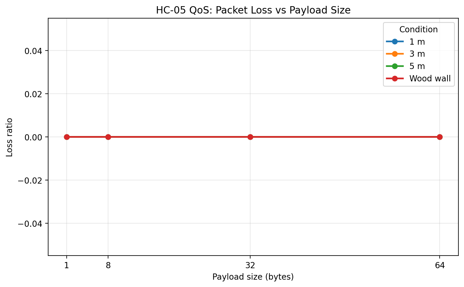
The combined condition-level summary is shown below. The 1 m baseline, 3 m, 5 m, and wood wall conditions all completed successfully with zero packet loss across all payload sizes.
| Payload | Condition | Successes | Loss | Mean RTT (ms) | Jitter SD (ms) | Goodput (B/s) | Max RTT (ms) |
|---|---|---|---|---|---|---|---|
| 1 B | 1 m | 100/100 | 0.0 | 41.25 | 7.08 | 24.22 | 71.34 |
| 1 B | 3 m | 100/100 | 0.0 | 40.85 | 8.45 | 24.46 | 71.29 |
| 1 B | 5 m | 100/100 | 0.0 | 48.42 | 12.09 | 20.64 | 97.35 |
| 1 B | Wood wall | 100/100 | 0.0 | 41.64 | 7.90 | 24.00 | 76.45 |
| 8 B | 1 m | 100/100 | 0.0 | 52.63 | 4.98 | 151.89 | 71.20 |
| 8 B | 3 m | 100/100 | 0.0 | 55.76 | 6.65 | 143.39 | 79.94 |
| 8 B | 5 m | 100/100 | 0.0 | 64.12 | 14.93 | 124.72 | 132.54 |
| 8 B | Wood wall | 100/100 | 0.0 | 56.82 | 8.52 | 140.70 | 98.91 |
| 32 B | 1 m | 100/100 | 0.0 | 101.38 | 3.79 | 315.51 | 121.13 |
| 32 B | 3 m | 100/100 | 0.0 | 104.95 | 7.43 | 304.81 | 149.91 |
| 32 B | 5 m | 100/100 | 0.0 | 112.52 | 15.63 | 284.32 | 182.49 |
| 32 B | Wood wall | 100/100 | 0.0 | 103.85 | 5.25 | 308.03 | 125.28 |
| 64 B | 1 m | 100/100 | 0.0 | 172.17 | 3.43 | 371.64 | 190.06 |
| 64 B | 3 m | 100/100 | 0.0 | 173.06 | 6.49 | 369.73 | 218.79 |
| 64 B | 5 m | 100/100 | 0.0 | 184.71 | 28.22 | 346.42 | 376.21 |
| 64 B | Wood wall | 100/100 | 0.0 | 172.67 | 4.35 | 370.56 | 193.71 |
Plots
Place the generated PNG files into your Jekyll image folder, for example assets/images/hc05-qos/, and update the paths if needed.
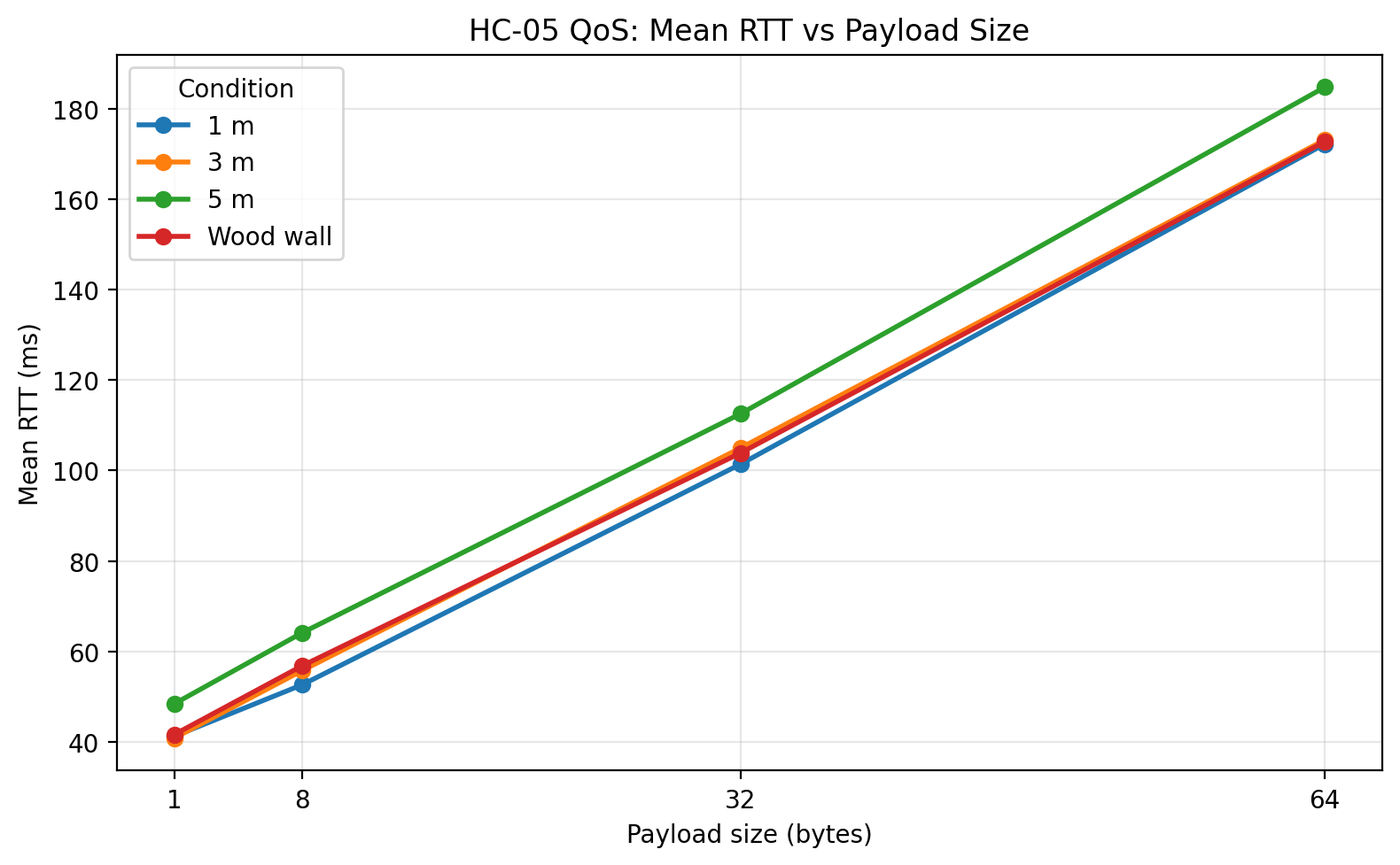
Mean RTT vs payload size
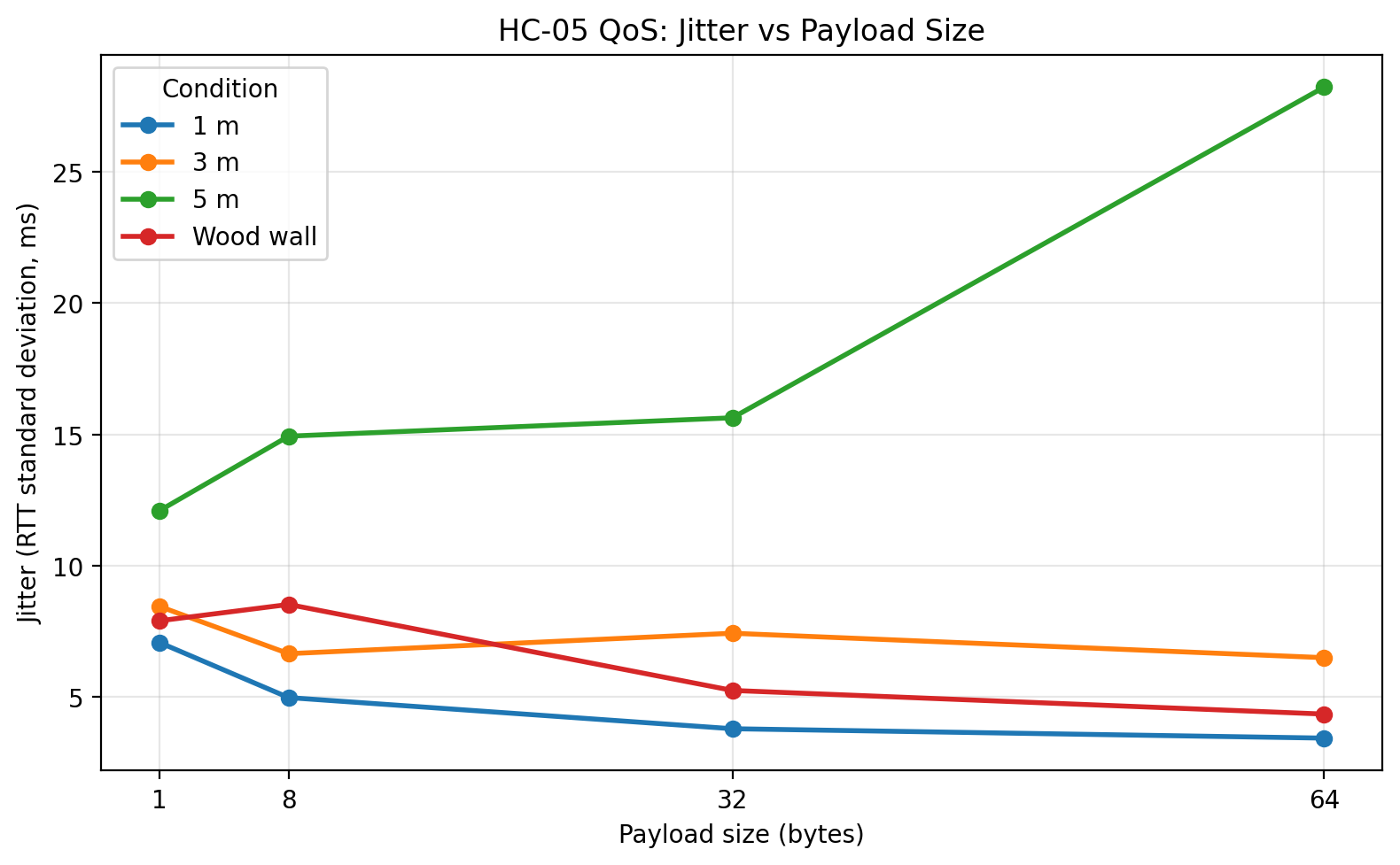
Jitter vs payload size
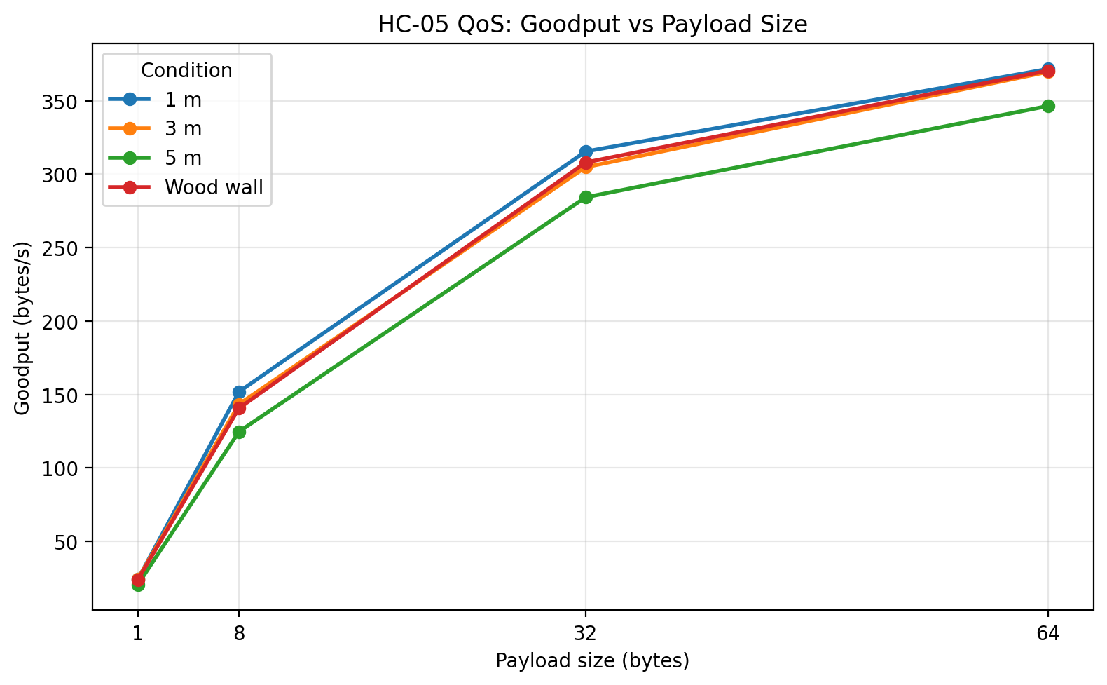
Goodput vs payload size
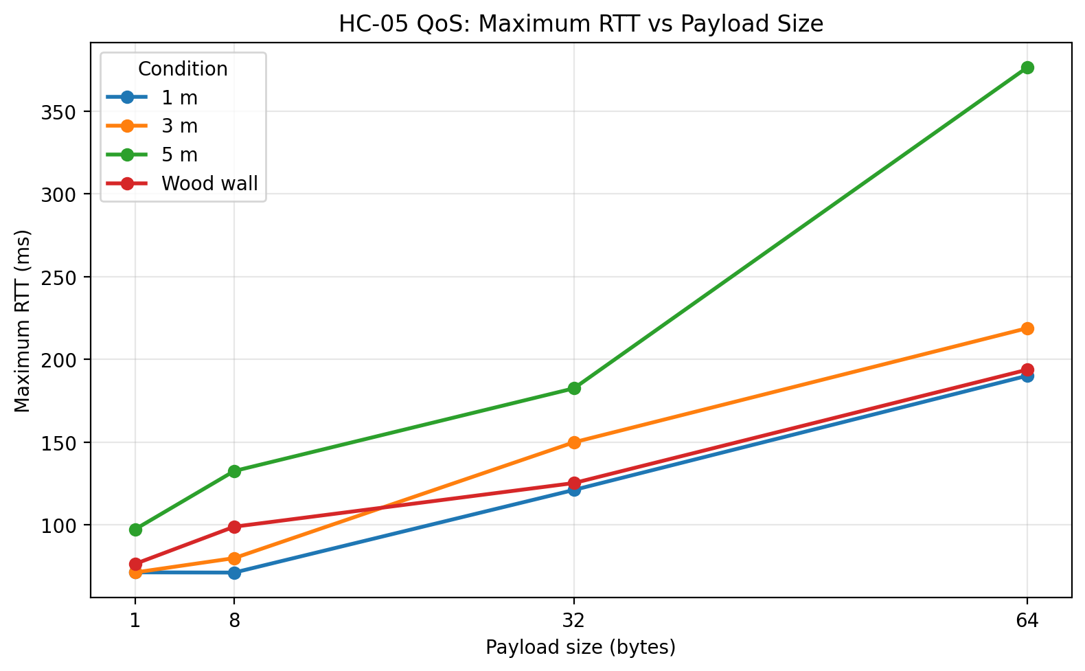
Maximum RTT vs payload size
Packet loss vs payload size
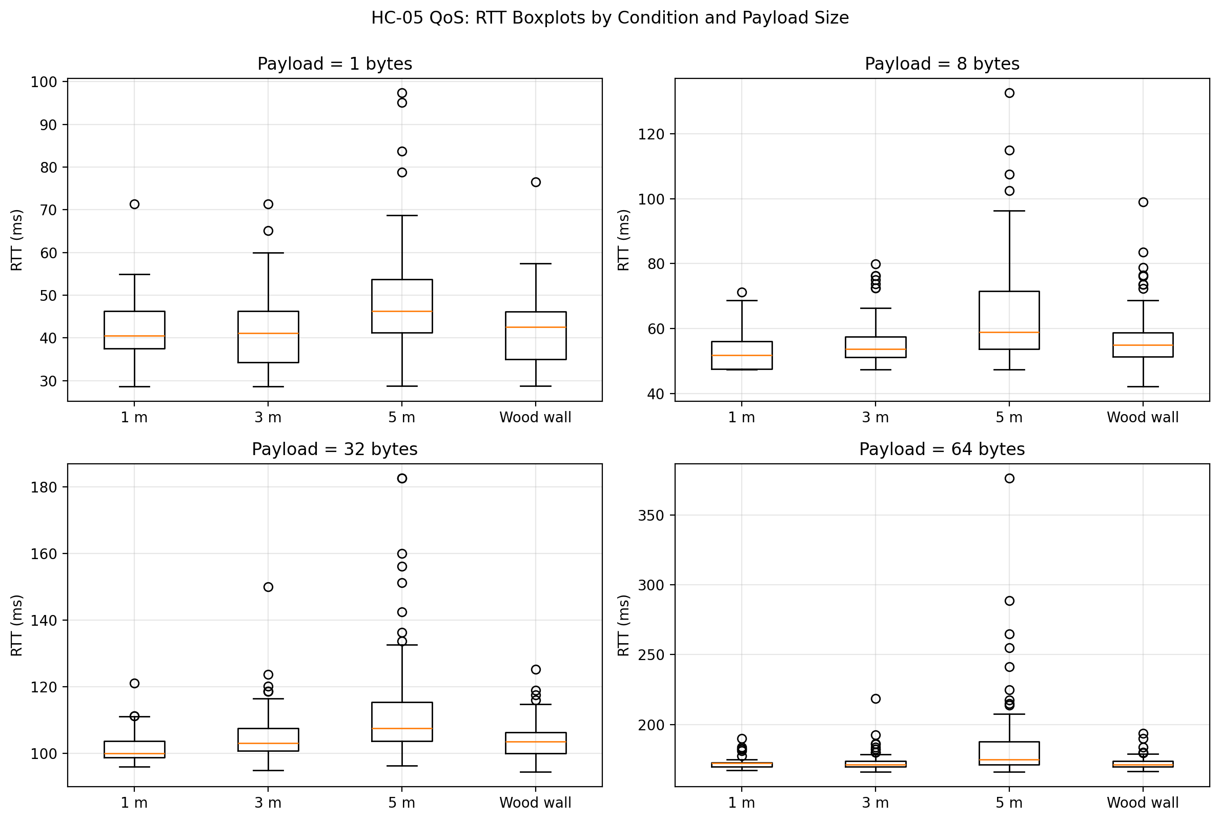
RTT boxplots by condition and payload size
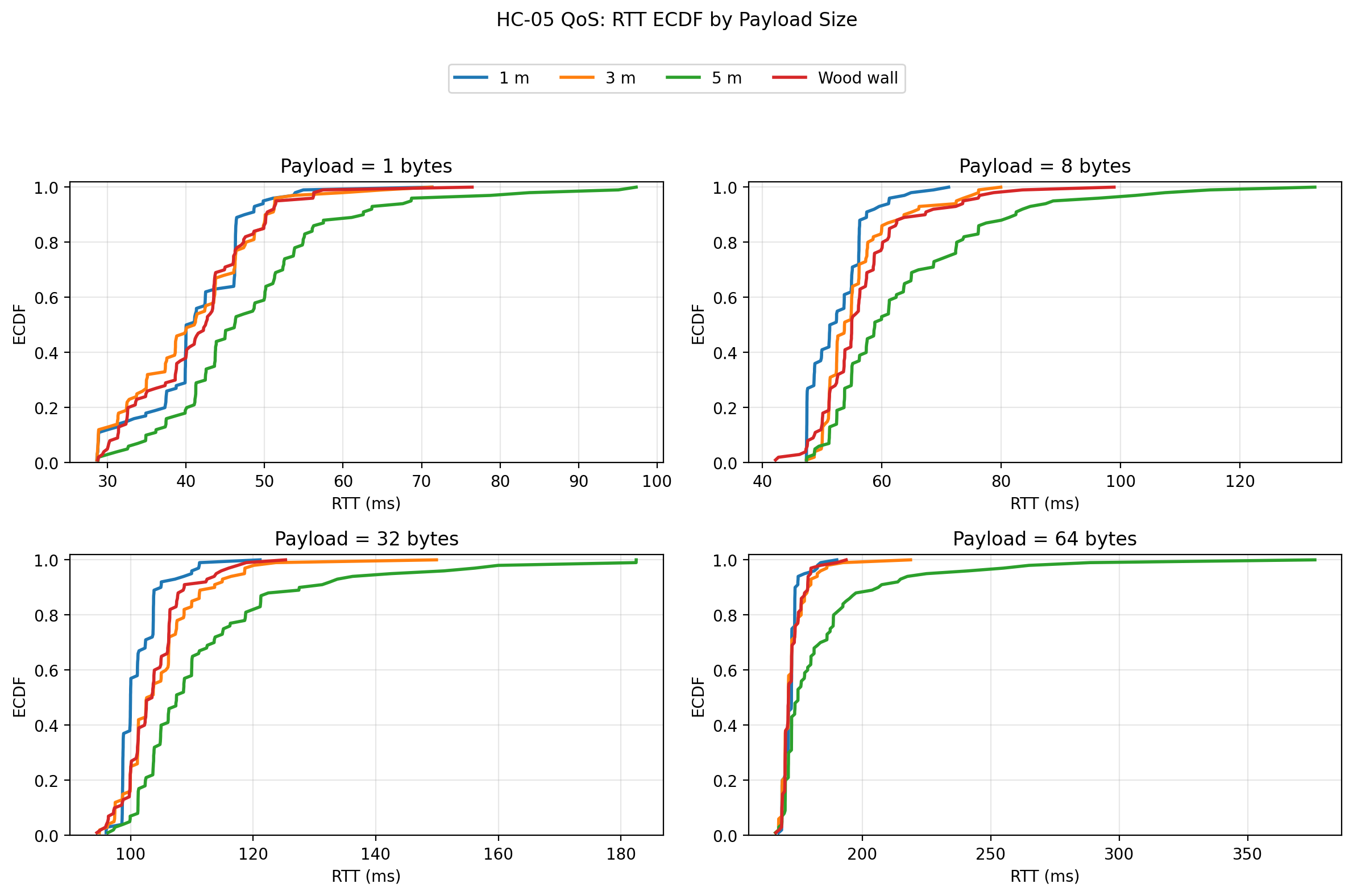
RTT ECDF by payload size
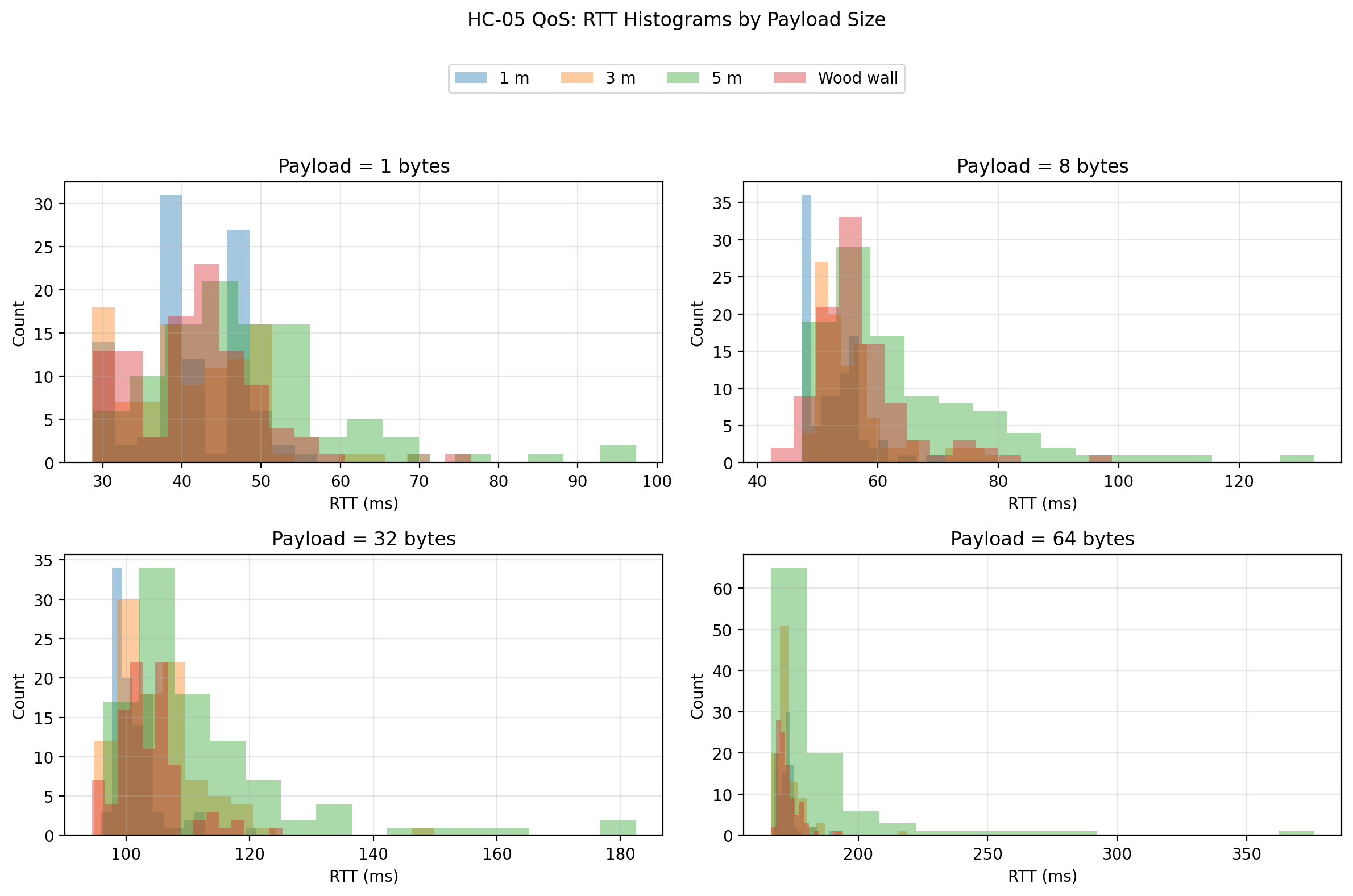
RTT histograms by payload size
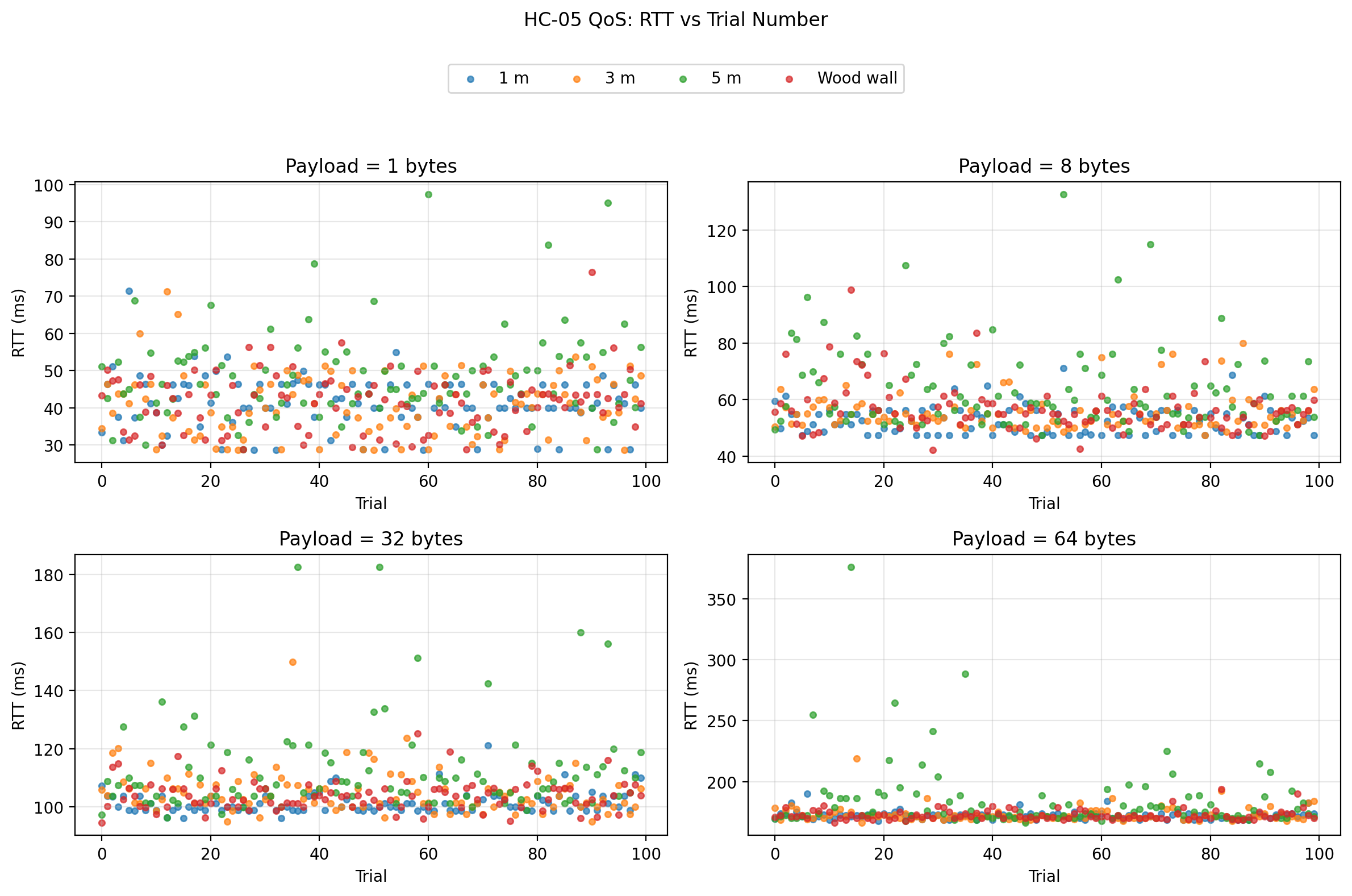
RTT vs trial number
Discussion
The first and strongest result is reliability. Across all tested conditions and payload sizes, the link returned 100% successful echoes. This means that under the tested indoor conditions, the system did not degrade by dropping packets. Instead, degradation appeared primarily as a timing phenomenon.
The second major result is the expected scaling of mean RTT with payload size. In every condition, RTT increased as payload size increased from 1 byte to 64 bytes. That pattern is exactly what a serial-bridge system should show, because larger payloads require more time to transmit over UART, more time to move through the Bluetooth serial profile, and more time to return through the same path. This indicates that the benchmark is capturing meaningful transport behavior rather than random noise.
The third major result is the behavior of goodput. Goodput increased strongly with payload size for every condition. This is also expected. Small packets spend a larger fraction of their total time in fixed overhead, while larger packets amortize that overhead more effectively. In this benchmark, the 64-byte payload delivered the highest goodput in all tested conditions, which makes it the most efficient of the tested packet sizes.
The fourth major result, and arguably the most interesting one, is the behavior of jitter. Distance had a much stronger effect on timing variability than on outright delivery reliability. The 5 m condition is where this becomes most visible. At 64 bytes, the mean RTT increased only moderately relative to the shorter distances, but jitter increased sharply and the worst-case RTT became much larger. In other words, the link remained connected and continued to return packets, but it became significantly less predictable. For an engineering discussion, that is important: the main degradation mechanism in this dataset is timing instability, not packet loss.
The wood wall condition behaved differently from the 5 m condition. Because the obstacle was a simple interior wood wall, it acted as a relatively mild barrier rather than a severe attenuation case. The wall condition stayed much closer to the 1 m and 3 m cases than to the 5 m case. That suggests that under these specific household indoor conditions, increasing distance to 5 m stressed the link more than inserting a single wood wall in the signal path.
The raw-data plots make this clearer than the summary statistics alone. The boxplots show that the 5 m condition produced visibly wider RTT distributions and more extreme outliers, especially at larger payload sizes. The ECDF plots show the 5 m curves shifted to the right, meaning a larger proportion of trials took longer to complete. The histograms reinforce that interpretation by showing longer right tails for the 5 m condition. Finally, the RTT vs trial scatter shows that the link did not exhibit a strong systematic drift over trial order; instead, the behavior was mostly stationary with occasional spikes, and those spikes were far more pronounced at 5 m than in the shorter-distance or wood-wall conditions.
From an engineering standpoint, these results suggest that the HC-05 + Uno combination is a viable short-range telemetry link for low-rate packet exchange, configuration traffic, or status reporting, but it should not be interpreted as a low-latency or tightly deterministic control link under all conditions. The absolute delay grows with payload size, and timing variability becomes increasingly important as conditions worsen.
What I would change in a next iteration
A useful next step would be to run the same benchmark at multiple UART rates, such as 9600, 38400, and 115200, while keeping everything else fixed. That would help separate serial-side limitations from Bluetooth-side limitations.
A second useful extension would be to repeat the experiment with another board while keeping the same HC-05 module and host laptop. That would make it possible to ask how much of the observed timing behavior belongs to the radio path and how much belongs to the embedded platform.
A third extension would be to move beyond stop-and-wait and test controlled streaming or burst behavior, though I would only do that after preserving this stop-and-wait baseline as a clean reference.
Final reflection
This benchmark began as a modest embedded communication project and developed into a useful systems experiment. The most important lesson was that communication quality should be measured, not assumed. A link that “works” can still behave very differently depending on packet size, distance, and the stability requirements of the application.
The final outcome was not just a Bluetooth demo. It was a reusable benchmarking setup with firmware, host tooling, and plotting scripts that can be extended to future comparisons. That makes it a much better engineering artifact than a simple point-to-point control example.